

Partial differential equations describe heat, flow and stress in every energy asset. Recast as energy-minimisation problems, they become natural targets for the Variational Quantum Eigensolver, and distributing it over networked quantum processors opens a path towards industrial-size simulations.
PDEs: the language of engineering
The temperature inside a reactor vessel, the stresses in a dam, the coolant flowing through a heat exchanger, the ions moving in a battery: engineers model them all with partial differential equations (PDEs). To solve a PDE numerically, space is cut into a mesh of N points, turning the equation into a large linear system Au = b or an eigenvalue problem Au = λu. Three-dimensional, multi-physics models of ageing over decades push N into the billions, and even the largest supercomputers must compromise on resolution.
Why a PDE solver is a VQE
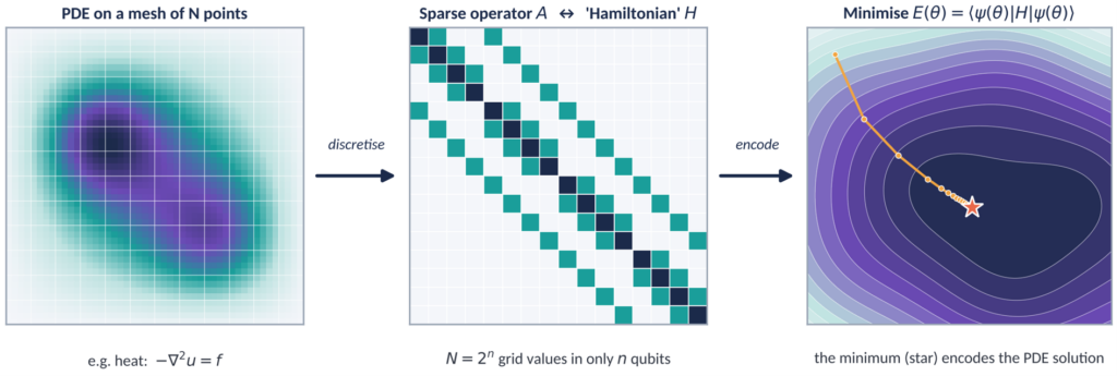
The Variational Quantum Eigensolver (VQE) was born in quantum chemistry. A quantum processor prepares a trial state |ψ(θ)⟩ with a parameterised circuit and measures its energy E(θ) = ⟨ψ(θ)|H|ψ(θ)⟩; a classical optimiser then adjusts θ to lower that energy. By the variational principle, the minimum is reached at the ground state of H.
Many PDEs share exactly this structure. The solution of the Poisson equation −∇²u = f, which governs heat conduction, electrostatics and elasticity, is the field that minimises a total potential energy. Once discretised, the sparse matrix A plays the role of the Hamiltonian and the solution is stored in the amplitudes of a quantum state (Figure 1). For eigenvalue problems, such as the neutron flux in a reactor core or the vibration modes of a structure, the link is even more direct: the fundamental mode is the ground state. Two features make this attractive: N grid values fit in only log₂N qubits (thirty qubits hold a billion-point field), and the discretised operator splits into a number of measurable terms that does not grow with the mesh. The art then lies in extracting the quantities engineers need, such as an average temperature or a peak stress, without reading out every amplitude.
Why distribute the VQE
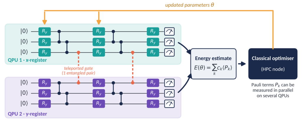
Finer meshes, more dimensions, more expressive circuits and error-mitigation overheads all demand more qubits than a single quantum processing unit (QPU) offers today. The VQE lends itself to distribution on two levels. First, the many terms of the Hamiltonian can be measured in parallel on different QPUs, with only classical communication. Second, the circuit itself can be split: in a 2D problem, the qubits encoding the x-coordinate sit on one QPU and those encoding y on another, linked by a few gates that consume entangled photon pairs delivered by Welinq’s quantum links (Figure 2). This is the quantum counterpart of domain decomposition, the classical HPC technique that spreads a mesh across compute nodes.
Welinq’s araQne compiler partitions the circuit and minimises the number of entangled pairs it needs. We co-design the variational circuits to be distribution-friendly from the start: richly entangling inside each processor, economical across them.
Momentum and outlook
Within the AQADOC project, we are building distributed VQE pipelines for model PDEs relevant to the energy sector, from heat diffusion and Poisson-type problems to eigenvalue problems, and benchmarking their accuracy against the number of QPUs and the entanglement budget. This work lays the foundations for running industrially meaningful simulations, such as the materials-ageing and structural questions raised by EDF, on the modular quantum computers now emerging.